
We pick up in this post the theme from the last – namely that one needs to look beyond a simple expectation value in order to assess the goodness of a ‘bet’. van der Wijst makes this point at the beginning of Chapter 3 by saying:
Recall that finance studies how people choose between risky future values. Risk means that the future outcomes of choices can deviate from their expected values. … Indeed, the variance (or its square root, the standard deviation) is the most frequently used quantitative measure of risk.
There is an interesting nuance here in that the variance of a statistically varying measurement is always expressed in units that are the square of the underlying units of the thing that is fluctuating. This can be a bit confusing when price is being considered because it isn’t obvious how to think about ($dollars)2. The alternative is to the standard deviation since it has the same units as the underlying entity but the downside (as we’ll see in some detail below) is that variances add linearly whereas standard deviations don’t. The compromise that seems work best (at least as suggested by van der Wijst) is the use of a percentage return rather than the price itself, where the return is defined as
\[ r_n = 100 \frac{p(t_n + 1) – p(t_n)}{p(t_n)} \; , \]
where the index $n$ tracks the particular element in a time series (e.g., $n = 7$ may mean the seventh business day of the time series which starts on Jul 31, 2025).
Defined in this way $r_n$ is dimensionless and so we sidestep the whole issue associated with the underlying units.
van der Wijst then gives a toy example to start off the connection between risk, return, and variance. In this toy example, there is a portfolio of two assets, $A$ and $B$, each with an possible return of $r_A$ and $r_B$, subject to some outcomes to be determined in the future. Note that I am deliberately avoiding using $r_1$ and $r_2$ as does van der Wijst to avoid clashing with the definition of $r_n$ given above; when I need to point to either ‘A’ or ‘B’ without directly specifying which I will use the index ‘i’.
Regarding the future outcomes, there are envisioned three possible scenarios with corresponding different returns for each asset. For clarity, the Scenarios will be labeled with the index ‘m’ when need arises to point to any (or all) of them without specifying which. Each scenario is equally likely to occur; in other words the probability for each scenario is exactly 1/3, which is denoted as ${\mathcal P}(S_m) = 1/3$.
The final ingredient is the fraction of the portfolio that is comprised of Asset A, $f_A$, and Asset B, $f_B$. For this example, the portfolio is made up of a 50-50 split between the two (i.e., $f_A = f_B = 0.5$).
With this information we can calculate the expected return for each asset across the various scenarios, given by
\[ E[r_i] = \sum_{m=1}^3 {\mathcal P}(S_m) \cdot r(S_m) \; \]
as well as the portfolio return for each scenario, given by
\[ r(S_m) = \sum_{i=A}^B f_i r_i(S_m) \; .\]
The table below summarizes both the individual returns per scenario for each asset, $r_i(S_m)$ (note it bears two indices – the ‘i’ to specify asset and the ‘m’ to specify scenario) along with $E[r_i]$ and $r[S_m]$ (in the margins).
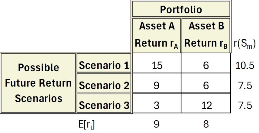
Regardless of which sum is performed first, by asset as
\[ E[\text{portfolio}] = \sum_{i=A}^B f_i E[r_i] \; \]
or by scenario as
\[ E[\text{portfolio}] = \sum_{m=1}^3 {\mathcal P}(S_m) r(S_m) \; , \]
the expected return of the portfolio is 8.5%
The picture isn’t complete without having a risk assessment and that means we want to calculate the variance of the portfolio. However, our task will be far simpler if we introduce some intermediate results.
First let’s calculate the variance of each asset across the scenarios, using
\[ \sigma^2[r_i] = \sum_{m=1}^3 {\mathcal P}(S_m) \left[ r_i(S_m) – E[r_i] \right] ^2 \; \] to arrive at
\[ \sigma^2[r_A] = \frac{1}{3} (15-9)^2 + \frac{1}{3}[9-9]^2 + \frac{1}{3}[3-9]^2 = 0.0024 \; \]
and
\[ \sigma^2[r_B] = \frac{1}{3} (6-8)^2 + \frac{1}{3}[6-8]^2 + \frac{1}{3}[12-8]^2 = 0.0008 \; .\]
Because variance involved squaring the underlying quantities we have reverted from percentages to floating point numbers since the only other alternative is to write these values as 24%2 and 8%2, with all the foreign-looking notation and mental gymnastics required to switch to dimensionless numbers.
The variance of the portfolio is given by
\[ \sigma^2[\text{portfolio}] = \sum_{m=1}^3 {\mathcal P}(S_m) \cdot \left[ r(S_m) – E[\text{portfolio}] \right]^2 \; . \]
Inserting the numbers from this toy problem gives
\[ \sigma^2[\text{portfolio}] = \frac{1}{3}(0.105-0.085)^2 + \frac{1}{3}(0.075-0.085)^2 \\ + \frac{1}{3}(0.075-0.085)^2 = 0.0002 \; .\]
Note that the variance of the portfolio is actually far lower than either the variance of asset A (by a factor of 12) or the variance of asset B (by a factor of 4). The question, of course, is why.
The answer lies in returning to the formula for calculating the portfolio variance and expanding the sums over the individual assets that make up $r(S_m)$. The calculation is a bit long and not terribly instructive and, moreover, it can be found in so many places, that I’ll just cite the result:
\[ \sigma^2(\text{portfolio}) = f_A^2 \sigma^2[r_A] + f_B^2 \sigma^2[r_B] + 2 f_A f_B \sigma[r_A,r_B] \; , \]
where the cross-correlation between assets A and B is given by
\[ \sigma[r_A,r_B] = \sum_{m=1}^3 {\mathcal P}(S_m) \left[ r_A(S_m) – E[r_A] \right] \left[ r_B(S_m) – E[r_B] \right] \; .\]
This cross-correlation term can be positive (increases the variance), zero (does nothing), or it can be negative (decreases the variance). Only in the latter case is the risk mitigated and the portfolio said to be diversified. In other words, diversification came about because Asset A was high in scenarios where Asset B was low and vice-versa (although not perfectly so). The cross-correlation term $\sigma[r_A,r_B] = – 0.0012$.
Next month, we’ll look at how to optimize the weights $f$ to produce a portfolio that balances risk versus return.